Ranking Resumes using Machine Learning

In this article we will see how machine learning can be applied to rank resumes.
Quick Summary
Its particularly challenging to rank 20 or more resumes even though the ranking is based only on 2 or 3 attributes. Recruiters often skip this step as it tends to be tedious and end up wasting a lot of hiring managers’ time. Its an error prone process if a junior recruiter is assigned the task.By automating resume ranking, we hope to avoid human error. We also hope to get early feedback and improved understanding of important attributes or top constraints by limiting the short list to top 3 resumes. Lastly it takes a few seconds for this crude Machine Learning program to rank 20 resumes- something that would take 10 minutes for an experienced recruiter. 
Disclaimer
This article covers a “Quick and Dirty” way to get started. This is no way the ultimate machine learning solution to the resume ranking problem. What I did here took me less than a day of programming. This could serve as an example for students of machine learning.
Problem Formulation
We train the machine learning program by using a “training set” of resumes which are pre-screened by a human expert. The resume ranking problem can be seen as a simple classification problem. We are classifying resumes into suitable (y=1) or unsuitable (y=0).  We know from machine learning theory that classification problems are solved by using the logistic regression algorithm.

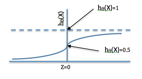
Sigmoid Function Showing Probability of a Resume being Suitable
We know the predictor function represents a value that lies between 0 and 1 as shown in the diagram above. The predictor or hypothesis function h_θ(X) is expressed as-
h_θ(X)=1/1-e^Z where z= θ^TX
where X is a vector of various features like experience(x₁), education(x₂), skills(x₃), expected compensation(x₄) etc. which decide if a resume is suitable or not suitable. The first feature x₀ is always equal to 1.

Features & Parameters
h_θ(X) can also be interpreted as the probability of the resume being suitable for  given X and θ. So the resume ranking problem is essentially solved by evaluating the function h_θ(X) with the resume yielding highest value of h_θ(X) getting the top rank.
With this prior knowledge of machine learning and logistic regression we have to find θ by studying a training set of resumes some of which were selected to be suitable -remaining ones being unsuitable.
Simplification of the problem
To further simplify the problem let us not bother about all the attributes like experience, education , skills, expected compensation, notice period etc. while ranking the resumes. As we saw in this earlier post ; we need to worry only about the top constraints. We selected the top constraints as those constraints which address “must have” features that are “hard to find”. Another benefit of limiting  these top constraints is that the same can be quickly and easily evaluated by the recruiters in short telephonic conversations with the candidates. This makes the process more efficient as it precedes and serves as a filter before the preliminary interview by the technical panel.
Decision Boundary
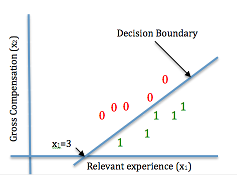
Training set is a set of resumes that are already known to be suitable or not suitable based on past decisions taken by the recruiters or hiring managers. Let us plot the training set for a particular opening based on past records. For the purpose of this article let us say that resumes are ranked only on the basis of 2 top constraints viz. relevant experience (x₁) expressed in number of years and expected gross compensation per month(x₂). The plot would look somewhat like what we see below.

Decision Boundary
If you draw a 45⁰ line cutting the X₁ axis at X₁=3, the same can be seen dividing the training set so that every point below the line represents a suitable resume and every point above it represents an unsuitable one. This line is machine learning terms is called the decision boundary. We can say that all the points on this line represent resumes where probability of them being suitable is 0.5.  This is also the point where z=0 as we have seen in the diagram above  showing the sigmoid function-
h_θ(X)=1/1+e^-(-3+x1-x2)=0.5
This equation represents a point on the sigmoid function where
Z=0   – replacing Z with θ^T X
θ^T X= 0
-3+X1+X2=0  – represents the Decision Boundary
Gradient Descent
Though we have visually plotted the decision boundary ; it may not be the best fit for the training set data. To get the best fit we can use gradient descent to minimize the error represented by the following equation-
 J(θ)=-1/m[_i=1∑^m y⁽ⁱ⁾*log(h_θ(x⁽ⁱ⁾) )– (1-y⁽ⁱ⁾)*log(1- h_θ(x⁽ⁱ⁾))] – where m is the number of instances in the training set and X⁽ⁱ⁾ is a vector representing x₀,x₁,x₂ for the i^th instance in the training set of resumes. y⁽ⁱ⁾ takes value 1 if the i^th instance was suitable and 0 otherwise. Here we are trying to minimize the function J(θ) by finding out a value of θ that minimizes the error function. Here θ is a vector of θ₀, θ₁and θ₂.
We can minimize J(θ) by iteratively replacing θ with new values as follows. Each iteration is  step of length α is for descending down the slope till we reach the minimum where the slope is zero.
θ_j:= θ_j-α(_i=1∑^m(h_θ(x⁽ⁱ⁾)- y⁽ⁱ⁾)* x⁽ⁱ⁾)
Implementation
We wrote the code to execute this in octave – as it’s a known bug-free implementation of machine learning algorithms and vector algebra. There are libraries available in Python and Java to build a more robust “production grade” implementation.
Limitations and roadmap for further work
The logistic regression algorithm is useful only if you have a reasonably large training set – at least 25 to 30 resumes. We also need to have the same selection criteria for the algorithms to work – hence you can’t reuse training sets across different job positions.  There are some “niche” positions where its impossible to find enough resumes- its both difficult and unnecessary to implement machine learning in such cases.
There are many “to-dos” before this program can be made useful. We need to use more features – particularly those which are “Must Have” types. We also need to have more iterations of the gradient descent with different values of  α . Lastly we need to have more resumes in the learning set to be able to further break it down into training set, validation set and test set.