Problems with Gradient Descent

Introduction

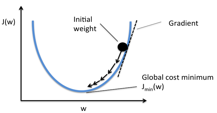
The objective of the optimization algorithm is to minimize the cost (J), to produce better and accurate predictions. In order to do so, the internal parameters, weights (w) and biases (b), need to be updated based on certain update rules or functions of the optimization algorithm.

Gradient Descent (GD) is one such first-order iterative optimization algorithm. It attempts to find the local minima of a differentiable function, taking into account the first derivative when performing updates of the parameters. The task becomes simple if the objective function is a true convex, which is not the case in the real world. In this article we will clarify why we need Gradient Descent, how it works, what are its shortcomings and what could be done about them.

An overview of how the learning takes place in Neural Networks

Link

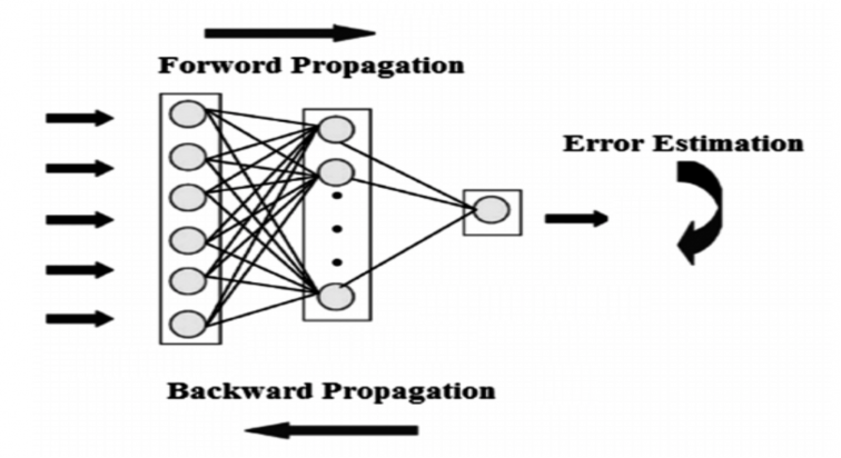
A neural network is a network of interconnected neurons comprising three ingredients – weights (w), biases (b), and activation functions. The learning process involves iterative forward and backward propagations.

Link

We propagate the input features forward in the network through various hidden layers, learning parameters (accounts for linear transformations) and activation functions (accounts for non-linear transformations), till we reach our final output layer. The predictions may differ from the actual values and hence we calculate loss J using a cost function which tells us how erroneous the predictions are.

This loss is propagated backwards across every layer while updating the learning parameters for each neuron in every layer of the network. This process is called back propagation.

^{w' =w − ηΔw
b' = b − bΔb
Where Δw = δJ/δw and Δb = δJ/δb}

The Problems:

When training a deep neural network with gradient descent and backpropagation, we calculate the partial derivatives by moving across the network from the final output layer to the initial layer. With the chain rule, layers that are deeper in the network go through continuous matrix multiplications to compute their derivatives.

In a network of n hidden layers, n derivatives will be multiplied together. If the derivatives are large, then the gradient will increase exponentially as we propagate down the model until they eventually explode, and this is what we call the problem of exploding gradient. Alternatively, if the derivatives are small, then the gradient will decrease exponentially as we propagate through the model until it eventually vanishes, and this is the vanishing gradient problem.

1. Vanishing Gradient
   

    

   If the range of the initial values for the weights is not carefully chosen, and the range of the values of the weights during training is not controlled, a vanishing gradient would occur which is the main hurdle to learning in deep networks. The neural networks are trained using the gradient descent algorithm:

   w' =w − ηδJ/δw

   Where J is the loss of the network on the current training batch. If the δJ/δw is very small, the learning will be very slow, since the changes in w will be very small. So, if the gradients vanish, the learning will be quite slow.
   
   The reason for vanishing gradient is that, during backpropagation, the gradients of inceptive layers are obtained by multiplying the gradients of concluding layers. So, let's say if the gradients of the concluding layers are less than one, their multiplication vanishes very fast.
   
   To summarize :

   • Gradient is the gradient of the loss function J with respect to each trainable parameter (weights w and biases, b).
   • Vanishing gradient does not mean the gradient vector is all zero (except for numerical underflow), but it means the gradients are so small that the learning will be very slow.
2. Exploding Gradient
   Exploding gradient occurs when the derivatives increase as we go backward with every layer during backpropagation. This is the exact opposite of the vanishing gradients.
   
   The architecture becomes unstable due to large changes in loss at each update step. The weights grow exponentially and become very large, and derivatives stabilize.
3. Saddle Point
   
   Saddle point on the surface of loss function is a point where, from one perspective, that critical point looks like a local minima, while from another perspective, it looks like a local maxima.
   Source : https://www.offconvex.org/2016/03/22/saddlepoints/
   
   Saddle point injects confusion into the learning process. Model learning stops (or becomes extremely slow) at this point, thinking that “minimum” has been achieved since the slope becomes zero (or very close to zero). From the other perspective though, this critical point is actually the maximum cost value. Saddle point comes into view when gradient descent runs in multidimensions.

The approaches to handle these problems:

I. Changing the architecture

This solution could be used in both the exploding and vanishing gradient problems, but requires good understanding and outcomes of the change. For example, if we reduce the number of layers in our network, we give up some of our model’s complexity, since having more layers makes the networks more capable of representing complex mappings.

II. Gradient Clipping for Exploding Gradients

Carefully monitoring and limiting the size of the gradients whilst our model trains is yet another solution. This requires some deep knowledge around how the changes could impact the overall performance.

III. Careful Weight Initialization

A more careful initialization of the model parameters for our network is a partial solution, since it does not solve the problem completely.

Conclusion:

• Converging to a local minima can be sometimes really slow, making the training costly.
• If there are multiple local minimas, then it’s highly probable that the algorithm may never converge to a global minima. This directly affects the model's performance

To handle these issues, there are several approaches that we can use such as proper initialization of model parameters, using the right activations functions, using optimal model architecture and choosing the right optimization algorithm (variation of GD as well as other optimizers).

About Encora